This document seeks to clarify some of the often misunderstood elements of Fault Tree mathematics. While not an exhaustive review, it covers the typical trouble areas.
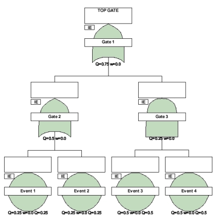
Two events under an OR gate, both using the same failure model. Two other events under an AND gate, both using another failure model. The OR and AND gates under an OR Top Gate. (We are not focusing on "w" results in this example, only Q).
Methods/Models Used
Quantification method: Rare
Fixed models:
![]() Model 1 for Event 1 and 2, Unavailability = .25
Model 1 for Event 1 and 2, Unavailability = .25
![]() Model 2 for Event 3 and 4, Unavailability = .5
Model 2 for Event 3 and 4, Unavailability = .5
Analysis: Retain results at all Gates
Cut Sets
"A cut set is a collection of basic events; if all basic events occur, the top event will occur." (Kumamoto/Henley, p. 227)
The cut set view from Gate 2: E1, E2 (two cut sets, each with one Event)
The cut set view from Gate 3: E3:E4 (one cut set with two Events)
Analysis
Begin by calculating the Unavailability of each cut set, using the number of Events in each. Then, at each Gate level, calculate the System Unavailability at that point, working your way up to the top. Remember though... you need to consider the view of the cut sets the Gate has looking down the tree. Not just the Q result at that level.
Cut Set Unavailability: ![]()
Where:
Qi = Event Unavailability
n = number of Events in the cut set.
Cut set #1 (E1): Q = .25 (due to only one event in the cut set)
Cut set #2 (E2): Q = .25 (ditto)
Cut set #3 (E3:E4): Q = .5 * .5 = .25
Next, calculate the Unavailability of the System at each Gate.
System (Gate) Unavailability: ![]()
Where:
n = number of cut sets under the Gate
Gate 2: Q = .25 + .25 = .5 (the Gate sees two cut sets)
Gate 3: Q = .25 (due to only one cut set)
Now, use the view of the cut sets from the Top Gate to calculate the overall System Q. In this tree, Gate 1 sees all three cut sets.
Cut set #1 (E1): Q = .25
Cut set #2 (E2): Q = .25
Cut set #3 (E3:E4): Q = .25
![]()
Top Gate 1: Q = .25 + .25 + .25 = .75
Interpretation
Note that the mathematics is completely focused on the cut sets. Additionally, the Q values at each Gate level are not simply OR'd or AND'd together.
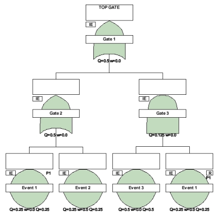
The subtle change in this example is that Event 1 has been repeated under Gate 3. This changes the cut set view from the Top Gate.
Methods/Models Used
Quantification method: Rare
Fixed models:
![]() Model 1 for Event 1 and 2, Unavailability = .25
Model 1 for Event 1 and 2, Unavailability = .25
![]() Model 2 for Event 3, Unavailability = .5
Model 2 for Event 3, Unavailability = .5
Analysis: Retain results at all Gates
Cut Sets
The cut set view from Gate 2: E1, E2 (two cut sets, each with one Event)
The cut set view from Gate 3: E3:E1 (one cut set with two Events)
Analysis
Cut Set Unavailability: ![]()
Where:
Qi = Event Unavailability
n = number of Events in the cut set.
Cut set #1 (E1): Q = .25 (due to only one event in the cut set)
Cut set #2 (E2): Q = .25 (ditto)
Cut set #3 (E3:E1): Q = .5 * .25 = .125
Next, calculate the Unavailability of the System at each Gate.
System (Gate) Unavailability: ![]()
Where:
n = number of cut sets under the Gate
Gate 2: Q = .25 + .25 = .5 (the Gate sees two cut sets)
Gate 3: Q = .125 (due to only one cut set)
Now, use the view of the cut sets from the Top Gate to calculate the overall System Q. In this tree, Gate 1 only sees the E1 and E2 cut sets due to the Repeat of Event 1. This is due to the absorption rule of minimal cut set analysis. (Kumamoto/Henley, p. 248)
"A minimal cut set is such that if any basic event is removed, it is no longer a set. A cut set that contains other sets is not a minimal cut set." (Kumamoto/Henley, p. 229)
The cut set E3:E1 is not a minimal cut set since it includes the cut set E1, due to the Repeat of Event 1. Therefore it is removed from the cut set analysis above the level of Gate 3.
Cut set #1 (E1): Q = .25
Cut set #2 (E2): Q = .25
![]()
Top Gate 1: Q = .25 + .25 = .5
Interpretation
Be careful of Repeat Events and Gates in your Fault Trees. Remember that they will cause cut sets to be removed from the analysis, perhaps causing you to doubt the validity of the results.
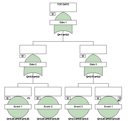
In this example Event 1 has been repeated, but Gate 3 is now an OR gate. This also changes the cut set view from the Top Gate.
Methods/Models Used
Quantification method: Rare
Fixed models:
![]() Model 1 for Event 1 and 2, Unavailability = .25
Model 1 for Event 1 and 2, Unavailability = .25
![]() Model 2 for Event 3, Unavailability = .5
Model 2 for Event 3, Unavailability = .5
Analysis: Retain results at all Gates
Cut Sets
The cut set view from Gate 2: E1, E2 (two cut sets, each with one Event)
The cut set view from Gate 3: E3, E1 (two cut sets, each with one Event)
Analysis
Cut Set Unavailability: ![]()
Where:
Qi = Event Unavailability
n = number of Events in the cut set.
Cut set #1 (E1): Q = .25 (due to only one event in the cut set)
Cut set #2 (E2): Q = .25
Cut set #3 (E3): Q = .5
Cut set #4 (E1): Q = .25
Next, calculate the Unavailability of the System at each Gate.
System (Gate) Unavailability: ![]()
Where:
n = number of cut sets under the Gate
Gate 2: Q = .25 + .25 = .5 (the Gate sees two cut sets)
Gate 3: Q = .5 + .25 = .75 (the Gate sees two cut sets)
Now, use the view of the cut sets from the Top Gate to calculate the overall System Q. In this tree, Gate 1 only sees the E1, E2, and E3 cut sets due to the Repeat of Event 1. This is due to the absorption rule of minimal cut set analysis. (Kumamoto/Henley, p. 248)
The cut set E1 is not a minimal cut set since it includes the cut set E1, due to the Repeat of Event 1. Therefore it is removed from the cut set analysis above the level of Gate 3.
Cut set #1 (E1): Q = .25
Cut set #2 (E2): Q = .25
Cut set #3 (E3): Q = .5
![]()
Top Gate 1: Q = .25 + .25 + .5 = 1
Interpretation
Again, the Repeat of an Event had an impact on the cut sets visible at the Top Gate, but so did the OR Gate 3. Event 3 (cut set) now appears at the Top Gate.
"Why is the Top Gate Q = 0?"
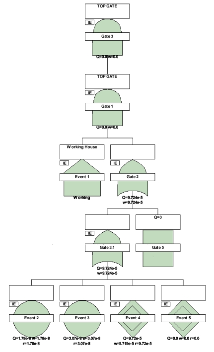
Answer: The Working House event (Q=0, R=1), when considered in the cut-set analysis for Gate 1, is the dominant force at this level in the FT. The cut set view from this gate is zero cut sets, resulting in Q=0. AND of a 0 results in a 0. If however, you change the Working House to a Failed House (Q=1, R=0), the model changes, resulting in Gate 1 having a non-zero value for Q. Additionally, the logic/failure models under Gate 5 need to be confirmed as it is providing Q=0 results as well. (In the real model, Gate 5 was a Transfer Gate.)
Working with Rate/MTTF models, and MTBF results can be confusing. In particular, the difference between the Mean Time To Repair and Repair Rate.
Rate Model:
Failure Rate = 1e-5 (one failure in 100,000 hours)
Repair Rate = 0
If the Repair Rate is 0, this assumes that no repairs are being made, and only one failure will occur during the lifetime of the device. MTBetweenF is then a very large number, and doesn't really exist because there is no time between failures since only one will happen.
MTTF Model:
Mean Time To Failure = 100,000 hours
Mean Time To Repair = 0
If MTTR = 0, this means that the repair is happening instantaneously. MTBF = MTTF + MTTR, so MTBF = MTTF in this case.
The point here is that you need to be careful of the value you assign to the Repair parameter. 0 can mean either a very short time, or a very long time, depending upon the model you are using.
Another misunderstood area is that of System Unreliability and Reliability. Commonly, people try to use the following simple formula:
![]()
While it is true for constant failure rates, it is not applicable for systems, which by nature, have a number of failure rates due to the various components that make up the system. It is not always possible to plug the system lifetime, and the calculated failure rate back into this equation and obtain the same value for R(t) that a program like ITEM Toolkit arrives at. (Kumamoto/Henley, p. 415)
Rather, when working with systems, the following equations should be used.
System Reliability: ![]()
System Unreliability: ![]()
Looking at these equations, you can see how the reliability of a system is based upon the Q (Unavailability) of the system, which from the first few examples in this document, you can see that is based upon cut sets.